8 Easy Google Sheets Functions Every Marketer Should Know
Learn simple Google Sheets tricks to analyse your marketing data easily. No Coding Needed!
Data Marketing in Google Sheets
Marketing is all about data. From customer behaviour to campaign performance, data tells the story that helps you make better decisions. If you want to explore and analyse this data easily without needing to know advanced programming languages like SQL or Python, the good news is you can! Google Sheets is a powerful tool that offers simple, intuitive query functions to help marketers like you get actionable insights from your data, and it’s FREE!
In this post, I’ll take you through a mini crash course on Google Sheets Query Functions. By the end, you’ll be able to run multiple basic types of statements and put them into practice right away. It’s surprisingly fun once you see the data insights you’ve been looking for appear in seconds!
Let’s get started! 🚀

Setting Up the Dataset
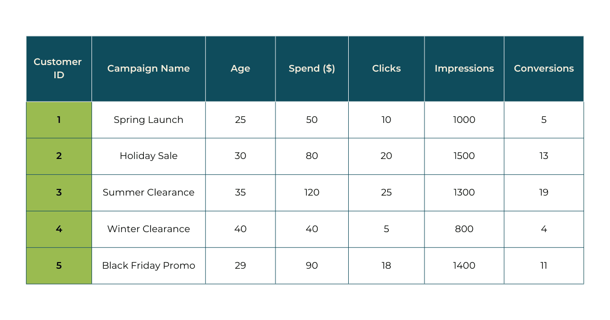
To make this hands-on, we’ll be using a small dataset of 20 rows that displays marketing campaign data. Copy the dataset to follow along.
Here’s what the top few rows look like:

Introduction to the =QUERY Formula in Google Sheets
Before we jump into specific examples, let’s start by understanding the basics of the =QUERY formula.
The QUERY function in Google Sheets is a powerful tool that allows you to retrieve and manipulate data from a range of cells, similar to a database query. With this function, you can filter, sort, and perform calculations on your data.
The general structure of the =QUERY function is:
=QUERY(data, query, [headers])
- data: This is the range of cells that you want to apply the query to (e.g., A1:H21). Typically, you can just highlight your entire table for this part.
- query: This is the condition or rule you’re applying to the data (e.g., selecting certain columns, filtering rows based on specific conditions).
- headers (optional): This specifies the number of header rows in the range. If you don’t specify this, Google Sheets assumes 1 header row.
Google Sheets Functions
1. SELECT Specific Columns (Basic Filtering)
The SELECT statement is the backbone of any query. It helps you pick specific columns from your data. It should always be enclosed by double quotes.
For example, if you want to see the Campaign Name and Spend of all customers, you can use this query:
=QUERY(A1:H21, "SELECT B, D")
This will return the Campaign Name (column B) and Spend ($) (column D).
Please note that the order of the columns matters. If you put ‘D’ before ‘B’, the output will be in that exact order.
2. WHERE Clause to Filter by Age Group
You can filter data with the WHERE clause, which is super helpful if you want to look at a specific subset of your data. For example, if you want to find customers aged under 30 to target younger audiences:
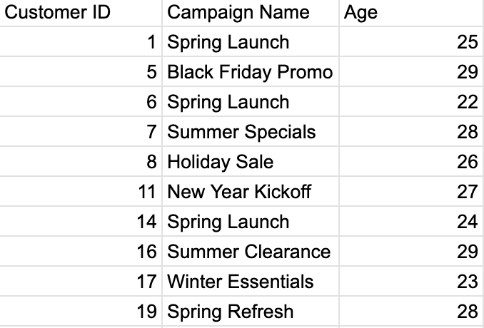
=QUERY(A1:G21, "SELECT A, B, C WHERE C < 30")
This isolates younger customers and their campaign preferences for targeted marketing.

3. Combine Conditions with AND/OR
To narrow down your search, you can use AND or OR to combine multiple conditions. For instance, to find Summer Specials and where the Spend is more than $60:
=QUERY(A1:H21, "SELECT B, D WHERE B = 'Black Friday Promo' AND D > 60")
Alternatively, if you want to find campaigns with more than 100 clicks or where spend exceeds $100:
=QUERY(A1:G21, "SELECT B, E, D WHERE E > 100 OR D > 100")
This helps prioritise campaigns with either high interaction or investment.
4. CONTAINS to Filter Campaign Types
The CONTAINS function is helpful for filtering rows based on whether a specific cell includes a keyword or phrase. This is especially useful when your data contains descriptive text, like campaign names, product categories, or customer segments.
Let’s say you want to analyse only the performance of “Winter Clearance” to understand its specific impact. You can use WHERE along with the CONTAINS keyword to filter your results.
=QUERY(A1:H21, "SELECT * WHERE B CONTAINS 'Winter Clearance'")
Contains with Multiple Conditions
You can also combine CONTAINS with AND or OR for even more targeted queries. For example, if you want to find specific campaigns, you could structure your query like this:
=QUERY(A1:G21, "SELECT B,D,G WHERE B CONTAINS 'Holiday Sale' OR B CONTAINS 'Spring Launch'")
5. ORDER BY to Rank Campaigns by Impressions
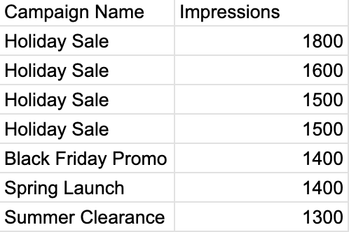
You can also order the data using the ORDER BY clause. If you want to see the campaigns with the highest visibility, you can sort by the impressions in descending order:
=QUERY(A1:G21, "SELECT B, F ORDER BY F DESC")
This will return the campaigns in order of highest spend first.

6. LIMIT BY Top Spending Campaigns
If you’re only interested in a limited number of results, you can use LIMIT. For example, to get the top 5 campaigns by spend:
=QUERY(A1:H21, "SELECT B, D ORDER BY D DESC LIMIT 5")
7. Aggregate Functions & GROUP BY
Google Sheets Query Functions also support aggregate functions such as SUM, AVG, COUNT, and more. For example, if you want to find the total spend per campaign, you can use the SUM function with a GROUP BY clause:
=QUERY(A1:H21, "SELECT B, SUM(D) GROUP BY B")
You must have at least one aggregate function for GROUP BY to work.
8. Arithmetic Operators for Total Conversions per Campaign
Google Sheets allows you to use arithmetic operators in queries. You can create new calculated columns easily to customise your reports. For example, to find the total conversions for each campaign:
=QUERY(A1:G21, "SELECT B, SUM(G) GROUP BY B")
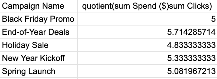
Another calculation you could do is the average spend per click for each campaign:
=QUERY(A1:G21, "SELECT B, SUM(D)/SUM(E) GROUP BY B")

These simple query functions allow you to get started with exploring your data. Google Sheets is an incredibly versatile and user-friendly tool, but it it does have its limits. As your marketing data grows, the complexity of the analyses you want to perform might outgrow its capabilities. Either way, it can do so much more than the above for data analysis and I encourage you to give it a try!
